Next: Quadratic Precision
Up: A NEM Interpolant for
Previous: Introduction
 NEM Interpolant
Farin [1] has proposed a
 interpolant based on Sibson's original
 natural neighbor interpolant.
By embedding
Sibson's coordinate in the Bernstein-Bézier
representation of a cubic simplex, a
interpolant is realized.
Bernstein-Bézier patches and related concepts
are widely used in surface approximations and in the
field of computer-aided geometric design [10].
A review article
on triangular Bernstein-Bézier surfaces can
be found in [11], while a
general treatment of multivariate polynomials over
multi-dimensional simplices is given by [12].
natural neighbor interpolant.
By embedding
Sibson's coordinate in the Bernstein-Bézier
representation of a cubic simplex, a
interpolant is realized.
Bernstein-Bézier patches and related concepts
are widely used in surface approximations and in the
field of computer-aided geometric design [10].
A review article
on triangular Bernstein-Bézier surfaces can
be found in [11], while a
general treatment of multivariate polynomials over
multi-dimensional simplices is given by [12].
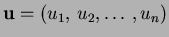
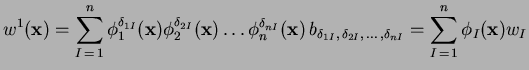
In what follows, multi-index notation
denoted by the bold characters
 and
and
 is used.
Multi-indexes are tuples of non-negative integers, the
components of which are subscribed starting at zero;
for instance,
is used.
Multi-indexes are tuples of non-negative integers, the
components of which are subscribed starting at zero;
for instance,
 . The
norm of a multi-index
. The
norm of a multi-index
 , denoted by
 , is
defined to be the sum of the components of
, namely
, is
defined to be the sum of the components of
, namely
 [10].
Let
[10].
Let
 , with
the property
, with
the property
 , be the
barycentric coordinate of a simplex
, be the
barycentric coordinate of a simplex
 .
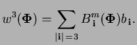
A Bernstein-Bézier surface of degree
.
A Bernstein-Bézier surface of degree  over the simplex
  can be written in
the form [12]
can be written in
the form [12]
 |
(1) |
where
 is known as the Bézier ordinate
associated with the control point
is known as the Bézier ordinate
associated with the control point
 . The control
net of
. The control
net of  is the network of
  -dimensional
points (
-dimensional
points (
 ). In Eq. (1),
 are -variate Bernstein polynomials in
  variables. To
elaborate, they are the terms in the multinomial expansion
of unity, i.e.
variables. To
elaborate, they are the terms in the multinomial expansion
of unity, i.e.
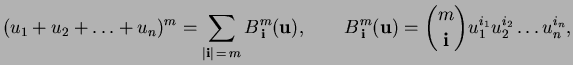 |
(2) |
where
 is the multinomial coefficient which
is defined as
is the multinomial coefficient which
is defined as
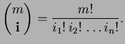 |
(3) |
The univariate linear Bernstein polynomials
are { ,
,  }, while the cubic polynomials are
{
}, while the cubic polynomials are
{ ,
,
 ,
,
 ,
,  }, where
![$ \xi \in [0, 1]$](img43.png) . Multivariate Bernstein polynomials have
properties very
much like their univariate counterparts. From the above
equations, some of the important properties of Bernstein polynomials
such as partition of unity, positivity, and cardinal interpolation,
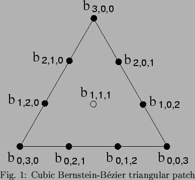
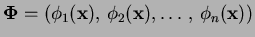
are easily inferred. The control points (circles) and associated
Bézier ordinate values (
) for
a cubic Bernstein-Bézier triangular patch are
shown in Fig. 2.
The interested
reader can refer to [13],
[11], and [10]
for further details on the properties and
applications of Bernstein-Bézier patches.
. Multivariate Bernstein polynomials have
properties very
much like their univariate counterparts. From the above
equations, some of the important properties of Bernstein polynomials
such as partition of unity, positivity, and cardinal interpolation,
are easily inferred. The control points (circles) and associated
Bézier ordinate values (
) for
a cubic Bernstein-Bézier triangular patch are
shown in Fig. 2.
The interested
reader can refer to [13],
[11], and [10]
for further details on the properties and
applications of Bernstein-Bézier patches.
Consider a point
 which has natural neighbors.
Let the Sibson coordinate of
which has natural neighbors.
Let the Sibson coordinate of
 be
be
 .
Since
.
Since
 ,
we note that
,
we note that
 can be considered as a barycentric
coordinate (non-unique) of the -gon in the plane. The
generalization of Bézier surfaces over a convex
polygonal domain was proposed by [14].
By using
instead of
can be considered as a barycentric
coordinate (non-unique) of the -gon in the plane. The
generalization of Bézier surfaces over a convex
polygonal domain was proposed by [14].
By using
instead of
 in
Eq. (1), we can
construct the surface [1]
in
Eq. (1), we can
construct the surface [1]
 |
(4) |
In the above equation, the Bézier ordinate
are associated with the control point
 , where
 are the projection
of the control points of the -variate Bézier polynomial
over the
are the projection
of the control points of the -variate Bézier polynomial
over the  -dimensional simplex onto the plane
[1]:
-dimensional simplex onto the plane
[1]:
 |
(5) |
On the basis of Eq. (5), one can infer that
the components of the barycentric coordinate
of the -dimensional
simplex is identical to that of the Sibson coordinate
of the mapped -gon on the plane.
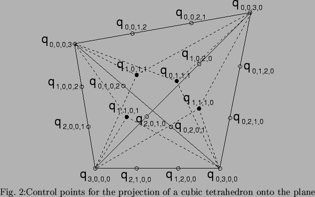
The connectivity rule for Bézier simplexes reflects the fact
that the domain simplex has all vertices connected to all
other vertices. If
and
 are two Bézier points
in the -gon simplex, then the rule indicates that
there must exist integers
are two Bézier points
in the -gon simplex, then the rule indicates that
there must exist integers  and
and  such that the multi-indexes
and
such that the multi-indexes
and
 satisfy
 |
(6) |
where
 denotes the multi-index having zero in all components except for the
 th component, which is one. The control points
for the projection of a cubic tetrahedron (
th component, which is one. The control points
for the projection of a cubic tetrahedron ( ,
,  ) onto
the plane is shown in Fig. 2.
) onto
the plane is shown in Fig. 2.
If we choose  in Eq. (4)
and let
in Eq. (4)
and let  denote the nodal function values, we
obtain
denote the nodal function values, we
obtain
 |
(7) |
which is the original Sibson interpolant.
Hence, Eq. (4)
can be viewed as a generalized form of the Sibson interpolant.
For ,
we arrive at the following
surface representation
[1]:
 |
(8) |
The above surface
form of a cubic Bézier -gon in Sibson coordinates is
used as the
NEM trial function for the
solution of fourth-order PDEs.
Subsections
Next: Quadratic Precision
Up: A NEM Interpolant for
Previous: Introduction
N. Sukumar