The
![]() interpolant has quadratic precison [1],
i.e. it can exactly reproduce a quadratic displacement field.
As opposed to
the above, the
interpolant has quadratic precison [1],
i.e. it can exactly reproduce a quadratic displacement field.
As opposed to
the above, the
![]() interpolant
proposed by [15] can only reproduce
spherical quadratics, i.e. functions of the form
interpolant
proposed by [15] can only reproduce
spherical quadratics, i.e. functions of the form
![]() . By virtue of the quadratic precision property,
the
. By virtue of the quadratic precision property,
the
![]() NEM interpolant can exactly represent
a state of constant curvature (second-derivatives of displacement)
which is required in order to pass the patch test
for a fourth-order PDE such as the biharmonic equation.
NEM interpolant can exactly represent
a state of constant curvature (second-derivatives of displacement)
which is required in order to pass the patch test
for a fourth-order PDE such as the biharmonic equation.
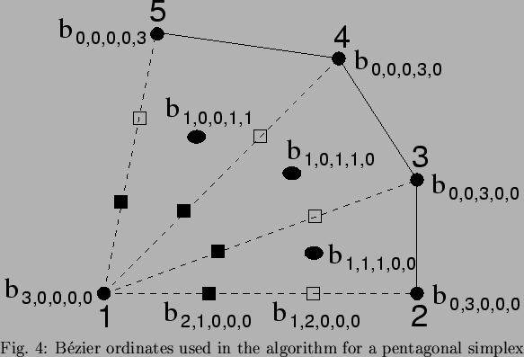
By judicious choice of the Bézier ordinates,
[16] realized a quadratic precision interpolant.
For a cubic ![]() -gon simplex, there are
-gon simplex, there are
![]() control points,
and consequently the
same number of Bézier ordinates. Of these,
control points,
and consequently the
same number of Bézier ordinates. Of these,
![]() control points lie along the
line joining vertices
control points lie along the
line joining vertices
![]() and
and
![]() .
The associated ``boundary'' Bézier ordinates to these
.
The associated ``boundary'' Bézier ordinates to these
![]() control points have either
one 3 and all other zeros (e.g.
control points have either
one 3 and all other zeros (e.g.
![]() for
for ![]() ) or
one 2, one 1, and other zeros (e.g.
) or
one 2, one 1, and other zeros (e.g.
![]() for
for ![]() ).
The former (vertex or corner ordinates) are equal to the
nodal function value, while the latter Bézier
ordinates are easily found in the tangent planes. The
additional
).
The former (vertex or corner ordinates) are equal to the
nodal function value, while the latter Bézier
ordinates are easily found in the tangent planes. The
additional
![]() ``free'' parameters are those which have three 1's and
all other zeros (e.g.
``free'' parameters are those which have three 1's and
all other zeros (e.g.
![]() for
for ![]() ). An optimal
choice for the center Bézier ordinate is given by
). An optimal
choice for the center Bézier ordinate is given by
![]() [16],
where
[16],
where ![]() is the centroid of the tangent Bézier ordinates
while
is the centroid of the tangent Bézier ordinates
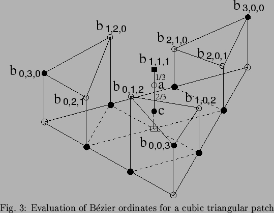
while ![]() is the centroid of the vertex (corner) Bézier
ordinates. The above choice of the center Bézier ordinate
guarantees quadratic precision. An illustration of
the calculation of the Bézier ordinates for a cubic triangular
patch is shown in Fig. 2.1. Referring to
Fig. 2.1, we can express
is the centroid of the vertex (corner) Bézier
ordinates. The above choice of the center Bézier ordinate
guarantees quadratic precision. An illustration of
the calculation of the Bézier ordinates for a cubic triangular
patch is shown in Fig. 2.1. Referring to
Fig. 2.1, we can express ![]() as
as
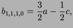 |
(9) |
 |
(10) |