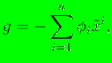
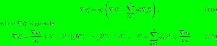
and therefore the gradient of  is
is
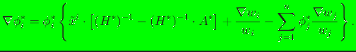 |
(13) |
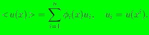
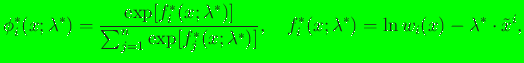
If the prior  is a Gaussian radial basis function
(see Reference [13]), then
is a Gaussian radial basis function
(see Reference [13]), then
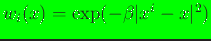 and Eq. (13) reduces to
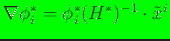 !
This result appears in the Appendix of Reference [12]. In
general,
!
This result appears in the Appendix of Reference [12]. In
general,
 depends on
 through
the expression given in Eq. (13).
The gradient of the basis functions is computed in
function dphimaxent().
through
the expression given in Eq. (13).
The gradient of the basis functions is computed in
function dphimaxent().
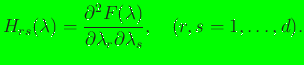
On taking the gradient of Eq. (13), we obtain the following
expression for the second derivatives of the max-ent
basis functions:
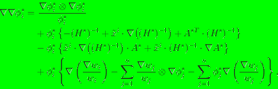 |
(14) |
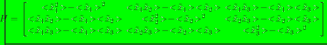
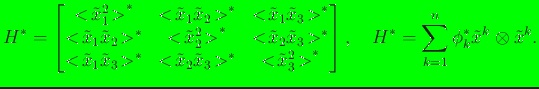
where on using the identity
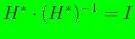 , the
gradient of the inverse of the Hessian
can be written as
, the
gradient of the inverse of the Hessian
can be written as
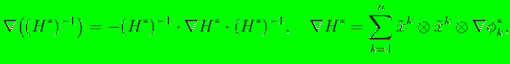 |
(15) |
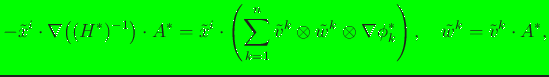
and therefore
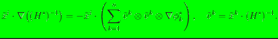 |
(16) |
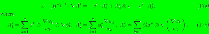
The term
 in Eq. (14) is given by
 |
(17) |
and the term
 is:
is: