


Next: Governing Equations and Weak
Up: A Note on Natural
Previous: Voronoi Diagrams and Delaunay
Natural Neighbor Interpolation
If  and
and  have a common boundary (
 -dimensional
face in
-dimensional
face in
 ),
),  and
and  are considered as
neighbors. The notion of a set of `neighboring nodes'
is generalized by the definition of natural-neighbor
nodes. The natural neighbors of any node are those in the
neighboring Voronoi cells, or equivalently, those to which
the node is connected by the sides of the Delaunay triangle.
The above definition extends if we are interested in finding
the natural neighbors of any sampling point
are considered as
neighbors. The notion of a set of `neighboring nodes'
is generalized by the definition of natural-neighbor
nodes. The natural neighbors of any node are those in the
neighboring Voronoi cells, or equivalently, those to which
the node is connected by the sides of the Delaunay triangle.
The above definition extends if we are interested in finding
the natural neighbors of any sampling point
 . By including
the sampling point
. By including
the sampling point  in the Delaunay triangulation,
the natural neighbors
of are the set of nodes which are connected to
it. It is noteworthy to point out that the number
of natural neighbors is a function of
position of
in the Delaunay triangulation,
the natural neighbors
of are the set of nodes which are connected to
it. It is noteworthy to point out that the number
of natural neighbors is a function of
position of
 , and depends on the local
nodal density.
, and depends on the local
nodal density.
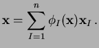
Consider an interpolation scheme for a function
 :
:
 , in the form:
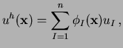 |
(2) |
where  (
(
 ) are the function values
at the
) are the function values
at the  natural neighbors, and
 are the weights (shape functions in FE)
associated with
each node. In the context of natural neighbor interpolation, the
weights
are taken as the n-n coordinates of the
point
in the plane. Natural-neighbor coordinates
were introduced by [1,2] and may be
defined in any number of dimensions. To illustrate, we use
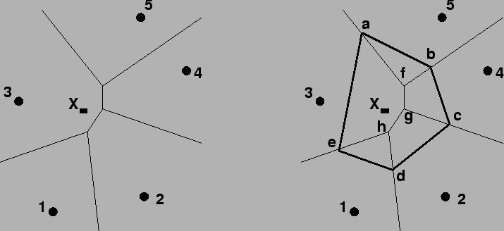
an example indicated in [9]. In Figure 1a,
five nodes and the sides of the Voronoi cells are shown. If
a point
is added in cell 3, then a new Voronoi cell can
be placed around it (see Figure 1b). The n-n coordinates of
with respect to a neighbor is defined as the ratio
of the area of their overlapping Voronoi cells to the total
area of the Voronoi cell about . For instance, in
Figure 1b,
are the weights (shape functions in FE)
associated with
each node. In the context of natural neighbor interpolation, the
weights
are taken as the n-n coordinates of the
point
in the plane. Natural-neighbor coordinates
were introduced by [1,2] and may be
defined in any number of dimensions. To illustrate, we use
an example indicated in [9]. In Figure 1a,
five nodes and the sides of the Voronoi cells are shown. If
a point
is added in cell 3, then a new Voronoi cell can
be placed around it (see Figure 1b). The n-n coordinates of
with respect to a neighbor is defined as the ratio
of the area of their overlapping Voronoi cells to the total
area of the Voronoi cell about . For instance, in
Figure 1b,
 is given by
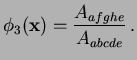 |
(3) |
The five overlapping regions in Figure 1b are known as
second-order Voronoi cells, while  is
a first-order Voronoi cell.
is
a first-order Voronoi cell.
Figure 1:
(a) Original Voronoi diagram for five ( ) neighboring nodes and ; (b) New Voronoi cell about (dark line)
 |
By the above definition of
, the
following two properties are self-evident:
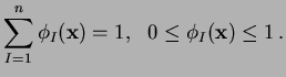 |
(4) |
Now, if were to coincide with any node, say node  for instance, then it is readily seen that
 and
and
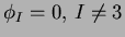 . Therefore the
n-n coordinates satisfy the Kronecker-delta property:
. Therefore the
n-n coordinates satisfy the Kronecker-delta property:
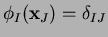 |
(5) |
and hence Eq. (2) is an
interpolation:
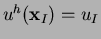 .
.
Since
is only non-zero in the union
of the circles that pass through the vertices of the
Delaunay triangles about node  , the n-n interpolation
is a local (interpolating) scheme. In addition, the
are continuosly differentiable
(
, the n-n interpolation
is a local (interpolating) scheme. In addition, the
are continuosly differentiable
( ) everywhere except at the nodes,
 , where all the derivatives are
discontinuous [1]. The proof of
the above in one-dimension is trivial. In 1D,
it is readily derived that the
, where all the derivatives are
discontinuous [1]. The proof of
the above in one-dimension is trivial. In 1D,
it is readily derived that the  are precisely
linear FE shape functions:
are precisely
linear FE shape functions:
 ,
,
 , where
 . Hence
FEM is realized (by the n-n interpolation) in 1D,
where it is well-known that the displacement derivative
is discontinuous at nodes (element
boundaries in 1D).
. Hence
FEM is realized (by the n-n interpolation) in 1D,
where it is well-known that the displacement derivative
is discontinuous at nodes (element
boundaries in 1D).
The natural neighbor coordinates
also
satisfies an important property known as the
Local Coordinate Property (LCP) -- geometrical coordinates
are interpolated exactly [1]:
 |
(6) |
Since the interpolant satisfies linear consistency, in the
context of elastostatics, the approximation (trial
function) can exactly represent rigid-body
motion and linear displacement fields.
Subsections
Next: Governing Equations and Weak
Up: A Note on Natural
Previous: Voronoi Diagrams and Delaunay
N. Sukumar