


Next: Implementation of the Natural
Up: Natural Neighbor Interpolation
Previous: Natural Neighbor Interpolation
In order to study a model PDE, let us consider
small displacement elastostatics, which is
governed by the equation of equilibrium:
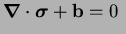 in in  |
(7) |
where
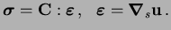 |
(8) |
In the above equations,
 is the
domain of the body,
is the
domain of the body,
 is the Cauchy
stress tensor,
is the Cauchy
stress tensor,
 is the small strain
tensor,
is the small strain
tensor,
 is the body force per unit volume,
 is the material moduli tensor,
 is the displacement,
 is the gradient operator, and
 is the symmetric gradient operator.
The essential and natural boundary conditions are
where  is the boundary of
  , and
, and
 and
and
 are prescribed displacements and
tractions, respectively.
are prescribed displacements and
tractions, respectively.
The weak form (principle of virtual work) is
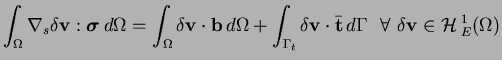 |
(10) |
On substituting the trial and test
functions in the above equation and using the arbitrariness
of nodal variations, the following
discrete system of equations is obtained:
 |
(11) |
where
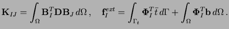 |
(12) |
In the above equation,
 is the shape function
vector and
is the shape function
vector and
 is the matrix of shape function derivatives.
Next: Implementation of the Natural
Up: Natural Neighbor Interpolation
Previous: Natural Neighbor Interpolation
N. Sukumar