Voronoi Diagrams and Delaunay Tessellations

The Voronoi diagram and its dual, Delaunay tessellation (covering of a surface with tiles) are geometric constructs that are widely used in the field of computational geometry. For simplicity, and for the purpose of illustration, we consider two-dimensional Euclidean space $\mathbf{R}^2$; the theory, however, is applicable in a general $k$-dimensional framework. Consider a set of distinct points (nodes) $P = \{ p_1 , \, p_2 , \ldots , \, p_N \}$ in $\mathbf{R}^2$. The tile (also known as Thiessen or Voronoi polygon) of $p_n$ is defined as [1]

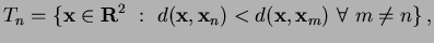$$T_n = \{ \mathbf{x} \in \mathbf{R}^2 \ : \ d(\mathbf{x},\mathbf{x}_n) < d(\mathbf{x},\mathbf{x}_m) \ \forall \ m \neq n \} \,,$$ (1)

where $d(.\, , \, .)$ is the Euclidean metric. Each tile $T_n$ is the intersection of finitely many open half-spaces, each being delimited by the perpendicular bisector (hyperlane in $\mathbf{R}^k$). In simpler terms, the tile $T_n$ can be viewed as the locus of all points closer to $p_n$ than to any other node. If $N = 2$, it is readily seen that the locus is the perpendicular bisector of the line joining the nodes, while if $N = 3$, the perpendicular bisector of the sides of the triangle ( $p_1,\,p_2,\,p_3$) which meet at the circumcenter of the triangle defines the Voronoi diagram. Generalizing, we see that the Voronoi diagram for a set of nodes divides the plane into a set of regions, one for each node, such that any point in a particular region is closer to that region's node than to any other node. The Delaunay triangles are constructed by connecting the nodes whose Voronoi cells have common boundaries. The Delaunay triangulation and the Voronoi diagram are dual structures -- each contains the same ``information'' in some sense, but represented in a different form. See [11] and [12] for details on Voronoi polygons. A nice exposition and comprehensive survey on Voronoi diagrams can be found in [13].